Organizing, cleaning, and normalizing (smoothing) cDNA microarray data

All product names are given as examples only and they are not endorsed by the USDA or the University of Illinois.

INTRODUCTION

The following is an interactive demo describing a set of programs we run to clean data before and after normalization. All programs are freely available and described below. The final data file is ready to be used as an input file for SAS. The SAS programs we run are explained on another page.
Click here for use SAS to analyze normalized cDNA microarray data DEAD LINK on real website, cannot find file; Also check for grammar

While scanning, we try to cover the dynamic range of the scanner. To do so, we aim for about one or two saturated spots per subgrid (or about 1 saturated for every 200-400 spots). Ideally one would have no saturated spots. However, if one scanned to avoid any saturation, many spots will be of very low fluorescence value and in the range that produces higher variation.
Click here for an example of a nicely scanned slide

After scanning one needs to use a program such as GenePix Pro to identify which pixels of the large scanned image correspond to a spot and to assign an ID and array coordinate to each spot. The spot finding software allows one to flag bad spots and will generate an output file providing columns corresponding to many different statistics of each spot (such as median intensity Cy3, median intensity Cy5, and flags). We do all the flagging manually, flagging only spots that are obviously bad (i.e. dirt, artifacts, or very high background that is clearly affecting the spot). We do not use background corrected values as non-specific binding to the slide coating does not equate to non-specific binding to DNA, so it is not often relevant (November 3, 2009lly obvious and one can flag those spots) CHECK LINK FOR GRAMMAR - something not right

Click here for images and further explanations on scanning, spot identification, and flagging. ON CLOUGHLAB WEBSITE, THIS LINK POINTS TO *THIS* PAGE

Please feel free to contact me with any questions or comments: Steve Clough: sjclough@illinois.edu

DOWNLOAD SOFTWARE AND FILES NEEDEDNovember 3, 2009November 3, 2009November 3, 2009 normalization. The normalization process is done using R/maanova. Click on each of the following PERL program names to download them. SOMETHING NOT RIGHT WITH THIS HEADER, ERROR ON CLOUGHLAB WEBSITE

merge_imputeblank1.pl
This program collects data from the spot finding output file and does pre-normalization processing and filtering. The program was written assuming one is using GenePix .gpr data files. If you use another spot finding program, you might need to modify the program code or column headers. The program is written to find columns by name: "F635 Median", "F532 Median", and "Flag". Program written by Min Li.

changeflagandbadspot.pl
This program deletes flagged or weak spots (lower than the negative control) and replaces that cell in the table with a period as SAS recognizes a "." as a missing value and takes this into account in its statistical calculations. For example, if 1 spot out of 4 reps is bad and has a "." instead of a value, SAS will conduct its calculations for that gene based on 3 reps, not 4. Program written by Min Li.

calculatingAverageIntensity.pl
This program provides a table of average intensities for each spot across all slides for a given RNA sample. The normalized average intensities are calculated after the normalization step and after removing flags and weak spots. In addition to providing intensity values, the program also tells how many slides had a valid value for each spot. Program written by Min Li.

SUMMARY TABLE OF DOWNLOADABLE PROGRAMS AND FILES

Click here to obtain a table summarizing these programs and the input and output files used or generated by these programs

DOWNLOAD DEMO FILE

Click here to obtain a demo data set of .gpr files that you may use to test and learn how to use these programs
Click here to obtain a demo "experimental design" file

DOWNLOAD PERL, MAANOVA, AND R

To run these analyses you will need to download the FREE programs PERL and R as well as the microarray analysis R/maanova package developed by the Churchill lab. The Churchill website (http://churchill.jax.org/index.shtml) has links to various documents related to R/maanova and the statistical analysis of microarrays.

PRE-NORMALIZATION PROCESSING AND FILTERING

1. CREATE DESIGN FILE

Click here to download the demo DesignFile.txt
You need a design table file that tells the programs what samples are on which slides, and to tell them which dye was used to stain each sample on a given slide. Below is an example of an experimental design and the design file that describes it.
Click here for more information on Experimental design



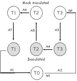In this experiment, RNA was extracted from 7 samples: Sample 1: Time T0 Sample 2: Time T3 mock inoculated Sample 3: Time T3 pathogen inoculated Sample 4: Time T2 pathogen inoculated Sample 5: Time T2 mock inoculated Sample 6: Time T1 mock inoculated Sample 7: Time T1 pathogen inoculated The samples were compared on a set of 7 slides or arrays (depicted as arrows, labelled A1-A7) following a loop design. The samples at the pointed end of the arrows were labelled with Cy5 and the samples at the other end with Cy3 dye.



Design table describing the above experiment:



Array	Dye	Sample
1	Cy3	1
1	Cy5	2
2	Cy5	3
3	Cy3	3
3	Cy5	4
4	Cy3	4
4	Cy5	5
5	Cy3	5
5	Cy5	6
6	Cy3	6
6	Cy5	7
7	Cy3	7
7	Cy5	1



This table describes an experiment with a single rep. For additional reps, just continue the table repeating the pattern and counting the repeats as new arrays. Below is a table that describes an experiment with two reps. Three reps would show 21 arrays, 4 reps 28 arrays, etc.



Array	Dye	Sample
1	Cy3	1
1	Cy5	2
2	Cy3	2
2	Cy5	3
3	Cy3	3
3	Cy5	4
4	Cy3	4
4	Cy5	5
5	Cy3	5
5	Cy5	6
6	Cy3	6
6	Cy5	7
7	Cy3	7
7	Cy5	1
8	Cy3	1
8	Cy5	2
9	Cy3	2
9	Cy5	3
10	Cy3	3
10	Cy5	4
11	Cy3	4
11	Cy5	5
12	Cy3	5
12	Cy5	6
13	Cy3	6
13	Cy5	7
14	Cy3	7
14	Cy5	1




NOTE: Save the design file as a tab delimited file in .txt format (i.e. DesignFile.txt).

2. PUT FILES IN SAME DIRECTORY

Put the PERL program merge_imputeblank1.pl and the appropriate soybean library used in the project (i.e. 18kA_format_demo.txt) into the same directory or folder (i.e. C:\temp\Demo). Note, if your study involved multiple libraries, you must run the analysis for each library completely separately from the other(s) from the beginning to the end (you will need a separate directory corresponding to each library). Although not essetial, put all the .gpr data files in the same folder for clarity (i.e. C:\temp\Demo\GPR_File).

3. SORT .GPR FILES

In order for the programs to know which files correspond to which arrays of the design file, the .gpr data files need to be named such that they can be sorted, and the sorting has to match your design file. Example based on the above design:


01_MS_0921_SB02.gpr (array #1, compares sample 1 to 2)
02_MS_0990_SB02.gpr (array #2, compares sample 2 to 3)
03_MS_0920_SB02.gpr (array #3, compares sample 3 to 4)
04_MS_0923_SB02.gpr (array #4, compares sample 4 to 5)
05_MS_0922_SB02.gpr (array #5, compares sample 5 to 6)
06_MS_0925_SB02.gpr (array #6, compares sample 6 to 7)
07_MS_0924_SB02.gpr (array #7, compares sample 7 to 1)
08_MS_0913_SB02.gpr (repeat of array #1, compares sample 1 to 2)
etc.

4. PRE-NORMALIZATION DATA PROCESSING

Run the program merge_imputeblank1.pl by double clicking on the program name which will open a window like the one below. This program will ask a few questions before it runs the analysis. After answering these questions, the program will merge all the .gpr data files and generate one table containing: location, gene IDs, 2 channel (Cy3, Cy5), and flag information for each array. In addition, all spots annotated as "blank" or "empty" are removed. This table will become the input file when using the R/maanova package to normalize the data.

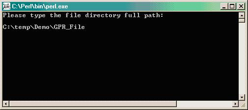
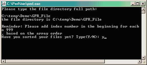
Double clicking merge_imputeblank1.pl gives this window:


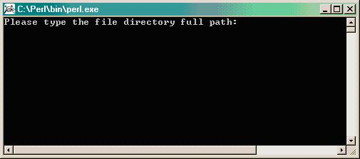
Type the path where files exist (i.e. C:\temp\Demo\GPR_File):


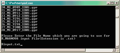
The program will verify the presence of the .gpr data files and will remind you to sort the files (done in Step 3 above), then you will be prompted to provide a file name for the new merged file that will become your input file for R/maanova (i.e. Rinput.txt).




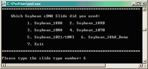
The program will ask for information on the soybean microarray library used. Note, if your study involved multiple libraries, you must run the analysis for each slide library completely separately from the other, from the beginning to the end of analysis. In this example, we used the Soybean_18kA_Demo library which is a smaller, modified version of the 18kA library.


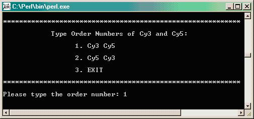
The program will ask for the order of Cy3 and Cy5 samples as reflected in your design table. In the example given in our design file above, the pattern starts with Array 1 where Sample 1 is Cy3 and Sample 2 is Cy5, so select "Cy3 Cy5" as the dye order.


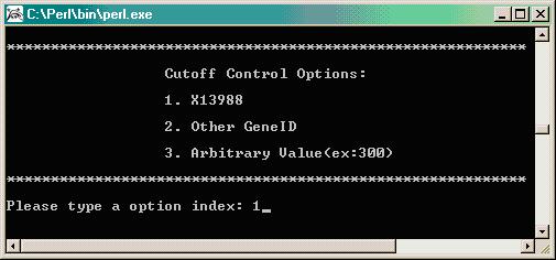
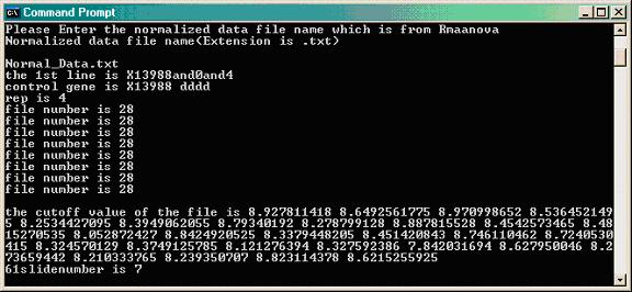
Next, the program will provide 3 options for establishing a minimum cutoff value. We found that the human control gene X13988 (Human Myosin Heavy Chain) acts well as a negative control on the soybean cDNA arrays and so we usually use this clone to establish the value at which to determine a minimum cutoff.
The program will average the X13988 values across each individual slide (both Cy3 and Cy5 values) to determine an average value for this negative control per slide. In the final analysis prior to running SAS, the program will remove all genes whose Cy3 and Cy5 average values (Cy3 + Cy5 / 2 for each spot) is less than the overall average on a given slide (Cy3 and Cy5 average for all 8 control spots of X13988 per slide) and will remove these spots from the statistical analysis. All flagged spot are converted to have both their Cy3 and Cy5 values equal the average value of the control X13988 as this will minimize the effects of a flag spot on the normalization calculation (the ratio for a flagged spot will be 1 instead of a possibly extreme value). All flagged spots are later removed from final input file. Note, one may also choose a different control ID by entering that control's GB ID, or one may pick an arbitrary value as the negative control cutoff value.


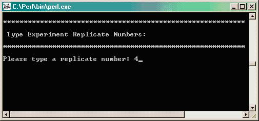
Enter number of replicates. In this experiment, RNA was extracted from 4 biological replicates.


Now the merge_imputeblank1.pl program will run and will generate a couple of files.

Rinput.txt

This is the file that you named at the start of merge_imputeblank1.pl program and contains all the data ready for R/maanova normalization.
flag_data.txt

Contains all spot flag information. This file will be needed for further imputation after R normalization to remove bad spots from data.
Summary_flags.txt

Contains listing of all bad flag spots.
rawdata_beforeBackgroundcorrection.txt

Contains raw data in format similar to that of Rinput.txt file.
rawdata_beforeBackgroundcorrection_noblank.txt

Same as the "rawdata_beforeBackgroundcorrection.txt" file except that the "Blanks" and "Empties" are removed.

RUNNING R/maanova TO NORMALIZE (SMOOTH) THE DATA

Note: the following descriptions and demo have been developed based on R version R 2.1.1.

Click here for the R/maanova functional codes. Once you are familiar with R/maanova this set of codes (called ".Rhistory") is all you'll need to run the normalization. DEAD LINK on real website, cannot find file .Rhistory

1. PUT FILES INTO SINGLE FOLDER/DIRECTORY

To run R, you need to have all the relevant files in the same folder/directory. Put the design file generated in step 1 (i.e. DesignFile.txt) and the merged file generated in step 4 (i.e. Rinput.txt) in the same directory (i.e. C:\temp\Demo\Normalization).

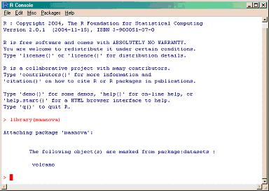
2. RUN MAANOVA PACKAGE IN R

The first step is to load the maanova library by simply typing:
>library(maanova)




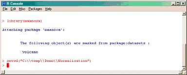
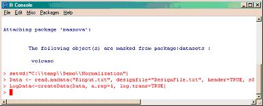
Set (identify) the working folder/directory where the data and design files are located using double backslashes (i.e. C:\\temp\\Demo\\Normalization)
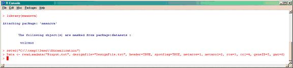
>setwd("C:\\temp\\Demo\\Normalization")




Read microarray experimental data (i.e. Rinput.txt and DesignFile.txt) into the program by typing:
>Data = read.madata("Rinput.txt", designfile="DesignFile.txt", header=TRUE, spotflag=TRUE, metarow=1, metacol=2, row=3, col=4, geneID=5, pmt=6)




Use createData() function to log2 transform the data into another file (i.e. a file named "LogData"). The number of reps is 1 because all clones are singly spotted on the 18kA slides except controls (and we do not average the control until after analysis).
>LogData = createData(Data, n.rep=1, log.trans=TRUE)




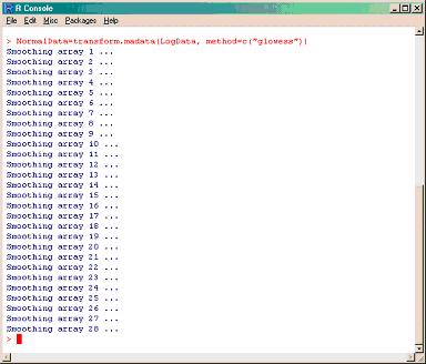
Normalize (smooth) the data with one of maanova's normalization methods. In this example we are using the "glowess" method. This intensity-based algorithm smoothes the scatter plot of Ratio (R/G) versus Intensity(R*G). Another popular normalization method is "rlowess" which is similar to glowess as it normalizes across intensities, but it also takes into account spatial effects. >NormalData=transform.madata(LogData, method=c("glowess"))




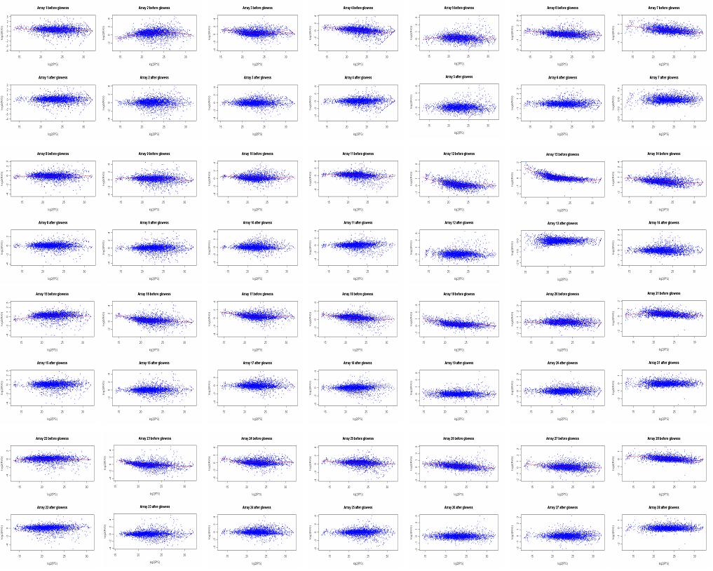
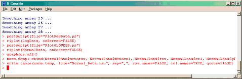
At the end of the smoothing, R will display a window for each set of scatter plots for a given slide, before and after normalization. One could save these images by copy/paste (ALT "Print Screen") window by window, or one can run a postscript function to save all the plots in two files, one will contain all plots before normalization, the other all the plots after normalization.

Images saved by copy/paste each window into PowerPoint. One can clearly see the smoothing effect of normalization (lower graphs) on the raw data (upper graphs).




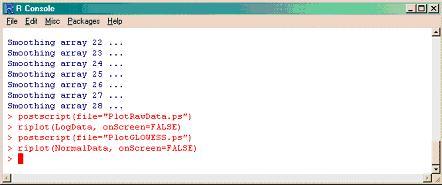
To save the Ratio intensity plots, before and after normalization, as a postscript file you need to define first the name of the .ps file with the postscript() function (i.e. PlotRawData.ps and PlotGLOWESS.ps) and then save them with riplot() function.
>postscript(file="PlotRawData.ps")
>riplot(LogData, onScreen=FALSE)




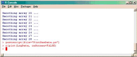
>postscript(file="PlotGLOWESS.ps")
>riplot(NormalData, onScreen=FALSE)




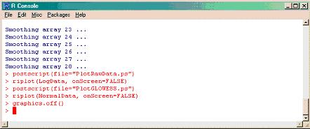
To close all the graphic windows, type:
>graphics.off()




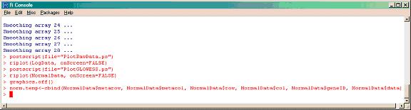
The location information, gene IDs, and the normalized data are combined in one temporary file in order to enable it to be saved later as an Excel file.
>norm.temp<-cbind(NormalData$metarow, NormalData$metacol, NormalData$row, NormalData$col, NormalData$geneID, NormalData$data)




To have this file in an Excel readable format, save the temporary file with the normalized data as a .csv file (i.e. Normal_Data.csv).
>write.table(norm.temp, file="Normal_Data.csv", sep=",", row.names=FALSE, col.names=TRUE, quote=FALSE)







POST-NORMALIZATION PROCESSING FOR SAS INPUT

1. FORMAT FILE
Save the newly generated file from R/maanova as a .txt file (i.e. Normal_Data.txt). Put this file and the previously made "flag_data.txt" file in the same directory along with the changeflagandbadspot.pl program (i.e. C:\temp\Demo).

2. IDENTIFY AND DELETE FLAG AND BAD SPOTS
Run the program changeflagandbadspot.pl to further impute the data. In this program, a "." is put in place of values that have been flagged. The program also uses the minimum cutoff value, as calculated during Pre-Normalization processes, to replace low values with a "." using the calculation (Cy3 + Cy5 < 2*median of control spot). In addition, it generates the replicatesforeachgene.txt file containing the number of valid replications for each spotted cDNA for an array across all replicates of that array. The program also generates a summary.txt file that is under construction + currently slunk.


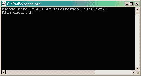
Double clicking changeflagandbadspot.pl gives this window.

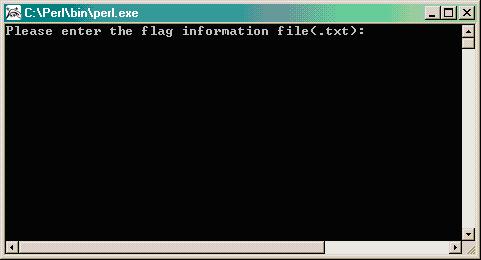
Type the name of the flag data file as it is in the same directory along with the PERL program (i.e. flag_data.txt); otherwise type the path where the flag data file exist.


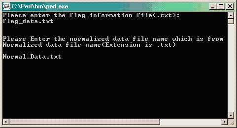
Type the name of the output normalized data file (R/maanova file) in format .txt (i.e. Normal_Data.txt). Hit ENTER and the program will run.




The program output files: forsasinput.txt and replicatesforeachgene.txt will be used during SAS analysis. These files should be saving in .csv format. To do so, open it in Microsoft Excel, and use the "Save As..." function to select .csv format.

3. CALCULATE AVERAGE INTENSITY
Run the program calculatingAverageIntensity.pl to calculate the average intensity value of every gene for every sample and the number of samples used for the calculation. Table also contains the average intensity value across the entire experiment and standard deviation as well as the stadard deviation divided by the experiment-wide average (which gives an indication of how much a given gene fluctuated throughout the experiment).

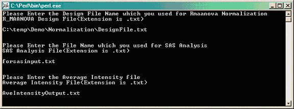
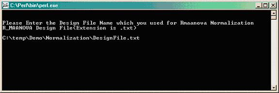
Double clicking calculatingAverageIntensity.pl gives this window.


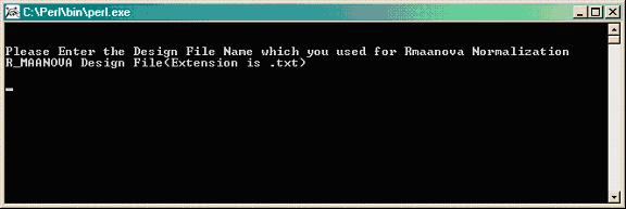
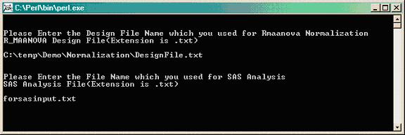
Type the path where the .txt design file is located, which was used for R/maanova normalization (i.e. temp\Demo\Normalization\DesigFile.txt).


Enter the name of the .txt file containing the normalized data for SAS input (i.e. forsasinput.txt).


Provide a name for your .txt output file (i.e. AveIntensityOutput.txt). Hit "ENTER" to run.